Analytic

grplot ships two standalone analytic functions in grplot.analytic.

---

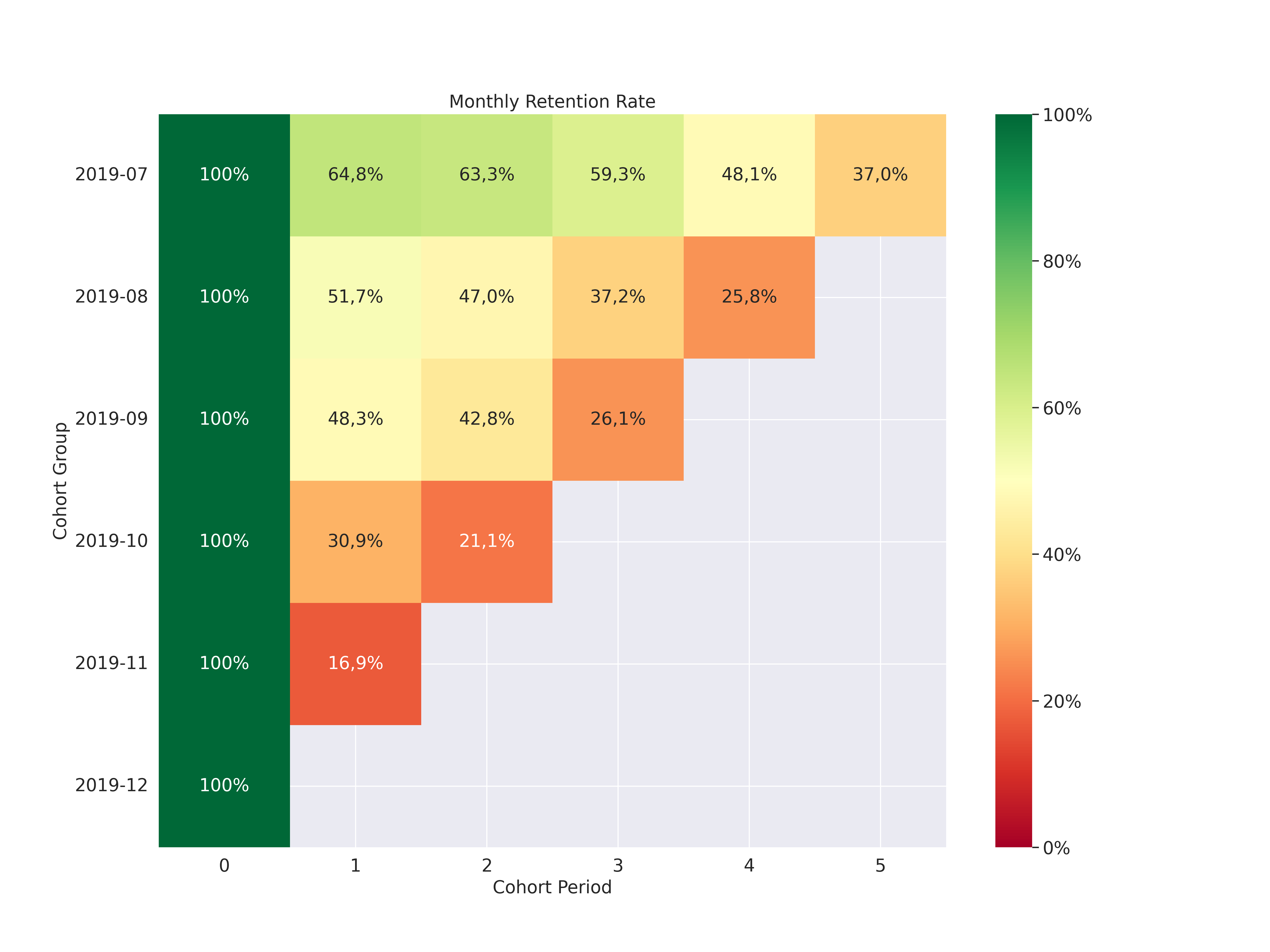
Cohort

Cohort retention analysis. Builds a monthly retention heatmap from a DataFrame containing a customer ID, a signup date, and a last-active date.

import: from grplot.analytic import cohort

Plot-Specific Parameters

customer_id (str)

Name of the column that uniquely identifies each customer.

signup_date (str)

Name of the column holding the first order / signup date (must be parseable as datetime).

last_active_date (str)

Name of the column holding the most recent active date (must be parseable as datetime).

display_summary (bool, default: False)

If True, display the intermediate cohort pivot table (cohort group × cohort period) alongside the heatmap.

Example

from grplot.analytic import cohort
import grplot_seaborn as gs
import pandas as pd

gs.set_theme(context='notebook', style='darkgrid', palette='deep')

df = pd.read_csv('https://github.com/ghiffaryr/grplot_data/raw/main/retail_raw_reduced.csv',
                 parse_dates=['order_date'])
df['last_active_date'] = df.groupby('customer_id')['order_date'].transform('max')
ax = cohort(df=df,
            customer_id='customer_id',
            signup_date='order_date',
            last_active_date='last_active_date',
            figsize=[16, 12],
            fontsize=16,
            sep='.',
            display_summary=True)

Rank Order, Gain, KS, and Lift

Rank Order table for binary classification model evaluation. Splits predictions into deciles (highest predicted non-event probability first) and computes cumulative Gain, KS statistic, and Lift for each decile.

import: from grplot.analytic import rank_order

Parameters

predict_proba (numpy.ndarray or pandas.DataFrame)

Predicted class probabilities with shape (n_samples, n_classes). Each row must contain the probability for every class; at minimum two columns are required. Pass the full output of sklearn’s predict_proba() directly.

true_label (list, numpy.ndarray, or pandas.Series)

Ground-truth binary labels with length n_samples.

class_non_event (int, default: 1)

Column index (0-based) in predict_proba that corresponds to the non-event class. For a standard two-class model where index 1 is the positive/non-event class, use the default value of 1.

display_table (bool, default: True)

If True, display the resulting rank order table in the notebook output before returning it.

Example

from grplot.analytic import rank_order
import numpy as np

np.random.seed(0)
predict_proba = np.array([np.random.uniform(low=0.1, high=1.0, size=10),  # class 0
                           np.random.uniform(low=0.1, high=1.0, size=10)])  # class 1
predict_proba = np.swapaxes(predict_proba, 0, 1)
true_label = np.random.randint(low=0, high=2, size=10)
rank_order_table = rank_order(predict_proba=predict_proba,
                              true_label=true_label,
                              class_non_event=1)

Decile	Minimum Prediction Probability	Maximum Prediction Probability	Mean Prediction Probability	Count Customer	Count Non-event	Count Event	Non-event Rate	Cummulative Count Customer	Cummulative Count Non-event	Cummulative Count Event	Cummulative Customer Percentage	Cummulative Non-event Percentage	Cummulative Event Percentage	KS	Lift
9	0.933037	0.933037	0.933037	1	1	0	100.0	1	1	0	10.0	14.29	0.00	14.29	1.43
8	0.883011	0.883011	0.883011	1	1	0	100.0	2	2	0	20.0	28.57	0.00	28.57	1.43
7	0.849358	0.849358	0.849358	1	1	0	100.0	3	3	0	30.0	42.86	0.00	42.86	1.43
6	0.812553	0.812553	0.812553	1	0	1	0.0	4	3	1	40.0	42.86	33.33	9.53	1.07
5	0.800341	0.800341	0.800341	1	0	1	0.0	5	3	2	50.0	42.86	66.67	-23.81	0.86
4	0.611240	0.611240	0.611240	1	0	1	0.0	6	3	3	60.0	42.86	100.00	-57.14	0.71
3	0.576005	0.576005	0.576005	1	1	0	100.0	7	4	3	70.0	57.14	100.00	-42.86	0.82
2	0.178416	0.178416	0.178416	1	1	0	100.0	8	5	3	80.0	71.43	100.00	-28.57	0.89
1	0.163932	0.163932	0.163932	1	1	0	100.0	9	6	3	90.0	85.71	100.00	-14.29	0.95
0	0.118197	0.118197	0.118197	1	1	0	100.0	10	7	3	100.0	100.00	100.00	0.00	1.00